
Continuous Charge Distribution | Electric Fields & Examples
Why is continuous charge distribution important?
In real applications, continuous distributions, where charges are spread continuously over a body, are important because of the large number of charges that are involved. For example, even 1 Coulomb of charge contains > 10^18 electrons. For convenience in calculations, instead of counting the charges individually, one considers continuous charge distributions. These are of three types: linear, surface, and volume charge distributions.
What does charge distribution mean?
A Charge distribution refers to the arrangement of charges in a system. It includes information about the charges and the locations of these charges. Charge distributions may be of two types. A discrete charge distribution consists of a collection of point charges, where each charge is considered as a separate entity, and the location of each charge is specified.
In a continuous charge distribution, the charges are spread out over a body, and the corresponding charge density may be uniform or non-uniform.
Recommended lessons and courses for you






Charges exert forces on each other, and the force between two point charges (discrete charges) {eq}Q_1 {/eq} and {eq}Q_2 {/eq} is mathematically expressed through Coulomb's Law as:
{eq}\mathbf{F} = k\,\dfrac{Q_1\,Q_2}{r^2}\mathbf{\hat{r}} {/eq} where the constant
{eq}k= \dfrac{1}{4 \pi \epsilon_0} = 9*10^9 \; N m^{2} C^{-2} {/eq} for free space, {eq}\epsilon_0 {/eq}, is called the absolute permittivity of free space.
In other dielectric media, the constant {eq}k =\dfrac{1}{4 \pi \epsilon} {/eq}, where {eq}\epsilon = \epsilon_0 \epsilon_r {/eq}, and {eq}\epsilon_r {/eq} is the relative permittivity of the medium.
The force is directed along the line joining the two charges; it is repulsive if the forces are of the same sign and attractive if they are of opposite signs.
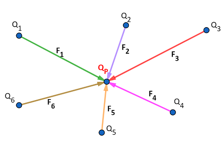 |
Fig. 1 shows a system of seven discrete charges.
The force due to the charges {eq}Q_i {/eq}, on the charge {eq}Q_P {/eq} are given by terms {eq}\mathbf{F_i}=k\,Q_i\,Q_P\,\mathbf{\hat{r_i}}/r_i^2 {/eq}, where i= 1 to 6.
The total force due to these 6 charges is then given by the principle of superposition as {eq}\Sigma_{n}\,(k\,Q_i\,Q_p/r_i^2 )\mathbf{\hat{r_i}} {/eq}, where {eq}r_i {/eq} is the distance between {eq}Q_p {/eq} and {eq}Q_i {/eq}, and {eq}\mathbf{\hat{r_i}} {/eq} is a unit vector along the direction of the force.
If, in this same volume of space, instead of 6 charges, there are 1000 charges, then the force acting on {eq}Q_P {/eq} is given by a similar summation over 1000 such terms.
If one keeps increasing the number of charges in this manner, at one stage, the charge distribution is no longer a discrete charge distribution, but instead becomes a continuous charge distribution.
Examples of Continuous Charge Distribution
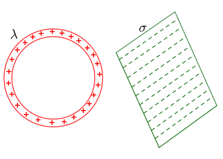
Fig. 2 gives a schematic representation of two types of continuous charge distributions, a one-dimensional charge distribution in the form of a positively charged metallic ring, and a two-dimensional negatively charged metallic plate. A continuous charge distribution can be considered as being made of many small pieces. Each small piece contains a very large number of charges.
 |
To calculate the total charge in each of these pieces, one requires the charge density of the distribution.
Continuous charges can be linear charges (such as on a line or ring), surface charges (such as on a plate), or volume charges (such as in a sphere).
For a line charge, the charge density is the charge per unit length {eq}\lambda {/eq}, for a surface charge, this is the charge per unit area {eq}\sigma {/eq}, and for a three-dimensional object such as a sphere, this is the charge per unit volume {eq}\rho {/eq}; The amount of charge in a small volume element {eq}\Delta V {/eq} is then {eq}\Delta Q = \rho(x,y,z)\Delta V {/eq}
The force magnitude between the charge elements from a continuous charge distribution and a point charge {eq}Q_P {/eq} is
{eq}k\,Q_P\,\Sigma \rho(r)\,\Delta V/r^2 {/eq}
In the limit {eq}n \to \infty {/eq}, where the division of elements is very fine and the pieces are very small, the sum changes to an integral, and the volume element is the infinitesimal {eq}dV {/eq}. In this limit, the force magnitude is
{eq}F_{cont}=k\,Q_P\,\int \rho(r)\,dV/r^2 {/eq}
These forces created by charged particles may be represented in terms of the Electric field (just as the Gravitational force may be represented by the Gravitational field).
For a system of two discrete charges, {eq}Q_1 {/eq} and {eq}Q_2 {/eq}, the charge {eq}Q_1 {/eq} creates an electric field around it {eq}\mathbf{E_1} {/eq}, and the charge {eq}Q_2 {/eq} experiences a force due to this electric field, which is given by {eq}Q_2 \mathbf{E_1} {/eq}.
Hence, from Coulomb's Law, the electric field magnitude {eq}E_1 {/eq} is {eq}E_1=k \dfrac{Q_1}{r^2} {/eq}.
Similarly, the charge {eq}Q_2 {/eq} creates an electric field around it, {eq}\mathbf{E_2} {/eq}, and the charge {eq}Q_1 {/eq} experiences a force {eq}Q_1 \mathbf{E_2} {/eq},
where {eq}E_2 = k \dfrac{Q_2}{r^2} {/eq}.
The direction of electric field and magnitude vary smoothly in space, allowing it to be represented through electric field lines:
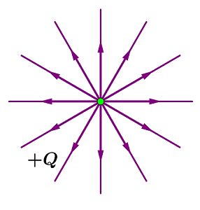 |
The field lines of a positive point charge are radially outward, as shown in Fig. 3, and those of a negative point charge are radially inward.
The direction of the electric field at a point is simply given by the tangent to the field line through that point.
Other properties of field lines include the following:
- They cannot intersect each other
- They start from positive charges and end at negative charges
- They do not form closed lines
- There is a higher density of electric field lines in regions with a high electric field and a weaker density of lines where the electric field is weaker
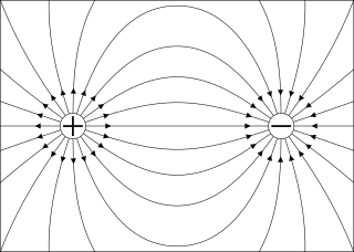
Some of these properties may be illustrated in Fig. 4, which shows the electric field lines of a dipole, which consists of a negative and positive charge of each magnitude, separated by a small distance.
 |
As for the force from a continuous charge distribution derived above, the electric field of a continuous charge distribution may thus be expressed for a volume charge distribution as:
{eq}\int \dfrac{k\rho(r)}{r^2}dv {/eq}
Calculating Electric Fields
(A) Discrete Charge Distribution
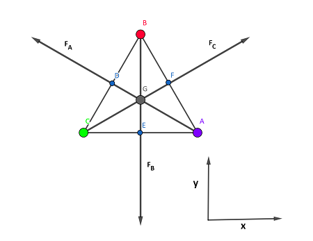 |
What is the electric field at the centroid of an equilateral triangle due to three positive charges {eq}Q_A {/eq} , {eq}Q_B {/eq}, and {eq}Q_C {/eq} at its three vertices?
The configuration is shown in Fig. 5, where the directions of the electric fields at the point G are given by the vectors {eq}F_A {/eq}, {eq}F_B {/eq}, and {eq}F_C {/eq}, respectively.
The side of the equilateral triangle is {eq}a {/eq}. The electric field values due to the three cases are:
{eq}E_A= k \dfrac{Q_A}{AG^2} {/eq} in the direction of AG
{eq}E_B= k \dfrac{Q_B}{BG^2} {/eq} in the direction BG, and
{eq}E_C= k \dfrac{Q_C}{CG^2} {/eq} in the direction of CG
Consider the right-angled triangle {eq}\Delta\, AFC {/eq}, with hypotenuse AC, where {eq}CF^2 + FA^2 = CA^2 {/eq} by Pythagoras' theorem.
{eq}FA = \dfrac{a}{2} {/eq} and {eq}CA = a {/eq}
Therefore, {eq}CF = \dfrac{\sqrt3}{2} a {/eq}
Also {eq}GC=\dfrac{2}{3}\, CF {/eq} as the point G is a centroid of an equilateral triangle.
Thus {eq}GC^2 = \dfrac{a^2}{3} {/eq} and so, {eq}GA^2 = \dfrac{a^2}{3} {/eq} and {eq}GB^2 = \dfrac{a^2}{3} {/eq}
Along the x-axis, the total electric field is given by {eq}-E_A sin(60^\circ)+E_C sin(60^\circ) {/eq}
Along the y-axis, the total electric field is given by {eq}-E_B + E_A cos(60^\circ)+E_C cos(60^\circ) {/eq}
Two special cases of this problem are
- When all three charges have equal values, the x- and y-components of the electric field are both zero, and the electric field at point G is then zero'.
- If the charges at A and C are equal, then the force along the x-axis is zero, and the direction of the resultant electric field is along the y-axis,
In this case, the electric field is simply:
{eq}E_A-E_B \\ =k \dfrac{Q_A}{AG^2}- k \dfrac{Q_B}{BG^2}\\ =k \dfrac{Q_A-Q_B}{AG^2} {/eq} where {eq}AG^2 = \dfrac{a^2}{3} {/eq}, as found above
(B) Continuous Charge Distribution
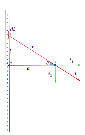 |
The electric field due to an infinite line charge at a location that is a distance d from the line charge may be calculated as described below:
The geometry of the problem is shown in Fig. 6,
Consider a line element at {eq}y=+l {/eq} on the wire, as shown.
The electric field due to this line element at P is expressed as
{eq}\dfrac{k \lambda dl}{r^2} {/eq}
This can be split into two perpendicular components, {eq}E_1 {/eq} and {eq}E_2 {/eq}, as shown in the figure.
{eq}E_1 = \dfrac{k \lambda dl}{r^2}cos(\theta) {/eq} and {eq}E_2 = \dfrac{k \lambda dl}{r^2}sin(\theta) {/eq}.
{eq}E_1 {/eq} is along the x-axis, and {eq}E_2 {/eq} is along the negative y-axis.
Consider another line element symmetrically, at {eq}y=-l {/eq}, below the origin.
This line element will contribute an electric field at point P, whose magnitude is {eq}\dfrac{k \lambda dl}{r^2} {/eq}.
The y-component of this field is opposite to the y-component of the field from the line element at {eq}y=l {/eq}, and thus the y-components of the electric fields of these two symmetrically placed elements cancel out
Their x-components add up, and the total electric field from the two elements is thus along the x-axis, and given by {eq}E_x=2 \dfrac{k \lambda dl}{r^2}cos(\theta) {/eq}
To find the total electric field due to the whole wire, all the line elements from {eq}-\infty {/eq} to {eq}\infty {/eq} have to be considered.
Thus the total electric field is {eq}E_{line} = \int_{-\infty}^{\infty} 2 \dfrac{k \lambda}{d^2 + l^2}\dfrac{d}{(d^2+l^2)^{1/2}} dl {/eq} since {eq}cos(\theta) = \dfrac{d}{r} {/eq} and {eq}r = (d^2+l^2)^{1/2} {/eq}, which simplifies to
{eq}E_{line} = 2 k \lambda d \int_{-\infty}^{\infty} \dfrac{dl}{(d^2+l^2)^{3/2}} {/eq}
This requires the value of the integral,
{eq}\int \dfrac{dl}{(d^2+l^2)^{3/2}}=\dfrac{l}{d^2 (d^2+l^2)^{1/2}} {/eq}
Using this formula and applying the limits of integration, the value of the electric field is obtained as
{eq}E_{line}=\dfrac{2 k \lambda}{d} {/eq}
The direction, as discussed above, is along the x-axis.
Coulomb's Law for continuous charge distributions gives the force magnitude between the charge elements from a continuous charge distribution and a point charge {eq}Q_P {/eq}
For a volume charge distribution, the force magnitude is
{eq}F_{cont}=k\,Q_P\,\int \rho(r)\,dV/r^2 {/eq}
Corresponding expressions for line charges and surface charges are given by:
{eq}F_{line}=k\,Q_P\,\int \lambda(r)\,dl/r^2 {/eq}
and
{eq}F_{surf}=k\,Q_P\,\int \sigma(r)\,ds/r^2 {/eq}
respectively.
Coulomb's Law gives the force between two point charges (discrete charges) {eq}Q_1 {/eq} and {eq}Q_2 {/eq} separated by a distance {eq}r {/eq} :
- {eq}F = k \,\dfrac{Q_1\,Q_2}{r^2} {/eq} where {eq}k=9*10^9 \; N m^{2} C^{-2} {/eq}.
The force between charges of the same sign is repulsive, while that between charges of opposite signs is attractive. For a collection of discrete charges {eq}Q_i {/eq}, where i=1 to n, the force on a charge {eq}Q_P {/eq} is expressed through a sum of forces due to the individual charges, {eq}Q_p\Sigma_{n}(k Q_i /r_i^2 ) {/eq}, where the {eq}r_i {/eq} is the distance between {eq}Q_p {/eq} and {eq}Q_i {/eq}.
The forces due to charged particles are represented through their Electric field. For a discrete system of charges, this is {eq}Q_p \Sigma_{n}(k Q_i /r_i^2 ) {/eq}. The smooth variation in electric field direction and magnitude allows it to be represented through electric field lines, where the direction of the electric field at a point is simply given by the tangent to the field line through that point. The following formulae represent the electric field of a continuous charge distribution with their corresponding charge densities:
- Volume Charge: {eq}\int \dfrac{k\rho(r)}{r^2}dV {/eq} for a charge density {eq}\rho {/eq}.
- Linear Charge: {eq}\int \dfrac{k\lambda(l)}{r^2}dl {/eq} for a charge density {eq}\lambda {/eq}.
- Surface Charge: {eq}\int \dfrac{k\sigma(s)}{r^2}ds {/eq} for a charge density {eq}\sigma {/eq}.
For a continuous charge distribution, the appropriate charge density must be considered.
Video Transcript
Electric Forces
Have you ever walked across a carpet in the wintertime and felt a spark of electricity when you touched a doorknob? Or have you had little pieces of lint or fuzz stick to your sleeve? These are examples of electric forces in action.
Electric forces are, quite simply, forces that are created by positive and negative electric charges. All electric charges exert a force on one another. Two charges that are both positive or both negative will repel one another. When one charge is positive and the other negative, they attract one another. We use the phrase ''opposites attract'' in all sorts of ways, but the phrase originated in the behavior of electric charges and the associated forces.
Electric Fields
Whenever we have two charges, we can treat one of them as a ''given'' and use the other as a ''test particle.'' We can move the test particle around in space and measure how much force it feels at each location. That force has both a magnitude and a direction. We can imagine drawing a little arrow at each location in space with the arrow's length proportional to the size of the force and the arrow's direction matching that of the force. When we're done, we'll have all of the space filled with little arrows. The whole collection is an example of a field.
A field is a set of values that specifies how some quantity depends on location, or perhaps on location and time. The field we're describing here is an electric field, and to make it match up with the official definition we must use a test particle that has a positive charge in the amount of one unit. Electric charge is measured in coulombs; so to do this imaginary test and wind up with the right and proper electric field, we need to use a test charge of +1 coulomb. So, in sum, an electric field is a map of the force that would be felt at any location by a +1 coulomb test charge.
If we draw all of these little arrows, we see that their size and direction change smoothly. We can play a sort of connect-the-dots game and draw continuous lines that follow the arrows. These are called electric field lines. The direction of our arrows will always be either toward the given charge (if it's negative), or away from that charge (if it's positive). The size of the arrows depends on the square of the distance between the two charges. If we double the separation, the size will go down by a factor of four. Things that behave this way are called ''inverse square law effects.''
Discrete Charge Distribution
What if we had two given charges, and our same +1 coulomb test charge? Now the test charge would feel a force from both of the other charges. Each piece would still be toward or away from the charge creating it, but when we add the two forces together we might get a total force in some other, different direction. The electric field created by the two charges will turn out to be the sum of the electric fields created by each one. This works for any number of given charges (a thousand, a million, even a billion). The arithmetic gets messier, but the idea stays the same. We can add up the pieces and draw our arrow based on the total.
So far, we've assumed that all of the charges are at precise little points in space. The test charge always has to be, since we want to find the field values at precise points in space. If the given charges are also at precise points, we call that a discrete charge distribution. In this context discrete just means ''at precise locations.''
Continuous Charge Distribution
A continuous charge distribution occurs when the given charge is spread out (evenly or unevenly) along a line, across a surface, or throughout a volume. In order to do calculations in such a situation, we have to have a mathematical expression that tells us how the charge is spread out. Instead of having x coulombs at a location, we will have x coulombs per unit length, or per unit area, or per unit volume. These are examples of charge densities. In general, the charge density doesn't have to be constant, it can vary depending on location.
Once we have that expression, we measure our electric field the same way. Each little bit of the charge distribution still exerts a force on the test particle, and we can still add those up, draw our arrows, and so on. Scientists do this by dividing the charge distribution up into a huge number of little pieces. For each piece, they figure out how much total charge is associated with that one piece by multiplying the charge density at that location by the length, area, or volume of the little piece, and then treating that like a point charge. They do this for every little piece, using the techniques of integral calculus. This basically finds the answer we'd get if the little pieces were so small they approached zero in size. Adding up all these little pieces gives us the total force on the test charge.
Coulomb's Law
Most of the time, scientists don't have to do measurements to find electric fields. There's a formula that gives the force between two charges.
F = (K)*(q)*(Q / r2)
In this equation, F is the force between the charges, q and Q are the charges in coulombs, and r is the distance between them in meters. K is a known constant of nature. So, given any charge distribution (discrete or continuous), scientists can do a bunch of math and find out exactly what the electric field is everywhere.
Lesson Summary
All right, let's now take a moment or two to review. All electric charges exert forces on one another. We learned that electric forces are, quite simply, forces that are created by positive and negative electric charges. The electric field is a map of the force that would be felt at any location by a +1 coulomb test charge. Remember that a field is a set of values that specifies how some quantity depends on location, or perhaps on location and time, and that electric fields can be visualized by continuous lines that follow the arrows, known as electric field lines.
We also learned that the charges creating the electric field can have a discrete distribution, if the given charges are at precise points, or a continuous distribution, if the given charge is spread out (evenly or unevenly) along a line, across a surface, or throughout a volume. Scientists calculate the field by treating the charge distribution as though it's composed of many point charges and adding up the field contributions using the techniques of calculus.
Register to view this lesson
Unlock your education
Become a Study.com member and start learning now.
Become a memberAlready a member? Log in
Go backResources created by teachers for teachers
I would definitely recommend Study.com to my colleagues. It’s like a teacher waved a magic wand and did the work for me. I feel like it’s a lifeline.
