Understand the differences between calculating the normal and the inverse normal distributions. Discover what the inverse cumulative distribution function represents. See examples of inverse Gaussian distribution or reverse bell curve.
Updated: 11/21/2023
Normal vs. Inverse Normal Distribution | Overview & Formula
Table of Contents
- What is Normal Distribution?
- Understanding Inverse Normal Distribution
- Inverse Cumulative Distribution Formula
- How to Calculate Normal Distribution and Inverse Normal Distribution Using GDC
- Lesson Summary
- FAQs
- Activities
Inverse Normal Probability: True or False Activity
This activity will help you assess your knowledge regarding the normal probability density function and the steps in calculating the inverse normal probability value.
Directions
Based on the given narrative, determine whether the following statements are TRUE or FALSE. To do this, print or copy this page on a blank paper and underline or circle the answer.
Helena weighs the frogs in a pond, obtaining a mean of 53 grams and a standard deviation of 8 grams. The weights followed a normal distribution, and there were 512 frogs in the population.
True | False 1. An inverse normal distribution is also known as a Gaussian distribution.
True | False 2. The sum of the probabilities of the frog weights would always be either 0 or 1.
True | False 3. An expression given as P(X < 53) can be composed as 1 - P(X > 53).
True | False 4. To know how many frogs are 80 grams or greater, Helena must use the concept of inverse normal probability.
True | False 5. The graph of the frog weights will trace a bell curve.
True | False 6. The standard deviation is depicted as the maximum point in the distribution of frog weights.
True | False 7. Helena can use the inverse normal probability only if the normal probability is unknown.
True | False 8. The given equation below is incorrect.
Answer Key
- False, because the correct statement is: A normal distribution is also known as a Gaussian distribution.
- False, because the correct statement is: The sum of the probabilities of the frog weights would always be 1.
- True
- True
- True
- False, because the correct statement is: The mean is depicted as the maximum point in the distribution of frog weights.
- False, because the correct statement is: Helena can use the inverse normal probability only if the normal probability is known.
- True
How do you find the inverse of a cumulative normal distribution?
Finding the inverse of a cumulative normal distribution involves determining the upper limit on a set of continuous outcomes in the normal distribution. The set of outcomes represents a specified probability that is transformed to a z-score via a z-table. The resulting z-score is then translated to the bound through the formula defining the z-score.
What does the inverse normal distribution tell you?
The inverse normal distribution illustrates how the probability of a continuous set of outcomes is related to the range for which those outcomes can occur. It transforms probability of the set to the bounds of the set.
How do you find the inverse of a normal distribution?
Finding the inverse of the normal distribution involves determining the range for a specific continuous set of outcomes within the normal distribution. To find the inverse, the probability of this set of outcomes is transformed into z-scores at each percentile of the range using a z-table. The resulting z-scores are then mapped to the bounds through the definition of a z-score. These resultant bounds precisely define the range.
Table of Contents
- What is Normal Distribution?
- Understanding Inverse Normal Distribution
- Inverse Cumulative Distribution Formula
- How to Calculate Normal Distribution and Inverse Normal Distribution Using GDC
- Lesson Summary
The normal distribution describes a distribution of probabilities that follow a well-defined behavior. Sometimes also referred to as Gaussian distribution or bell-curve distribution, the normal distribution helps determine the likelihood of a range of possibilities, rather than a single outcome. Two factors determine the characteristics of the distribution; which are mean {eq}(\mu) {/eq} and standard deviation {eq}(\sigma) {/eq}. These are effectively the most likely outcome and how likely it is for a result to deviate from that outcome.
In general, the normal distribution is generated by the equation:
{eq}f(X) = \frac{1}{\sigma \sqrt{2\pi}} e^{-\frac{1}{2}\left(\frac{X - \mu}{\sigma}\right)^2} {/eq}
 |
The probability of an event occurring within a range is defined by the integral of the normal distribution function bounded by that range. So in the range from arbitrary bounds, a to b, the probability is written:
{eq}P(a < X < b) = \int_{a}^{b} f(X) dX {/eq}
Taking the integral under the entire curve, which has the range {eq}(-\infty, \infty) {/eq}, yields a result of 1.
However, taking the integral over arbitrary intervals each time is computationally difficult and altogether impractical. Instead, calculating such a probability can be done much easier through the use of the z-score (or standard score). This z-score essentially defines the amount of standard deviations away from the mean that a particular outcome is. It is useful as a tool for directly converting between outcome and probability, and is defined by:
{eq}Z = \frac{X - \mu}{\sigma} {/eq}
It is important to note that a value of {eq}Z = 0 {/eq} corresponds to the outcome, X, being equivalent to the mean.

Your next lesson will play in
10 seconds
Where the normal distribution aims to calculate the probability of an event given an outcome, the inverse normal distribution formula provides a method for determining an outcome given a probability. Z-scores provide the best tool for performing both operations. The relations between Z and P are defined in "z-tables" which provide a direct, numerical conversion between the two concepts. It does not represent a formula but serves as a look-up tool that works in both directions. A useful program for generating z-tables is Microsoft Excel; The "NORMSDIST()" and "NORMSINV()" functions provide conversions from z-score to probability and the reverse respectively.
For the inverse distribution formula, given a probability of an outcome within an unknown range {eq}(-\infty, X) {/eq}, the z-score can be found from a z-table by looking up that particular probability (or the closest value to it); or in Excel by: {eq}Z = NORMSINV(P) {/eq}. After which, the bound, X, can be calculated by:
{eq}X = Z\sigma + \mu {/eq}
The cumulative distribution defines the probability of an event, X, occurring below a certain bound, a, in a normal distribution. The cumulative distribution formula can be written formally as:
{eq}P(X \leq a) = \int_{-\infty}^{a} f(X) dX {/eq}
 |
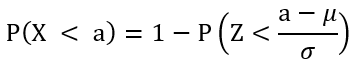
Since the entire area under the normal distribution curve is known to be 1, it is also possible to find the area under the curve of everything greater than the bound a through:
{eq}P(X \geq a) = 1 - P(X \leq a) {/eq}
Furthermore, the formula for a probability between two finite bounds can be re-written as:
{eq}P(a < X < b) = P(X < b) - P(X < a) {/eq}
The process of determining the cumulative distribution probability makes excellent use of the z-score conversion, avoiding integration. By finding the z-score associated with a, and then converting with the z-table, it immediately returns the associated probability. The probability can also be written with Z directly, by:
{eq}P(X \leq a) = P(Z \leq \frac{a - \mu}{\sigma}) {/eq}
The inverse cumulative distribution formula is simply the previous process put into reverse. Given a particular probability of an event occurring below an unknown bound a, Z can be immediately retrieved through a z-table, and converted to a through: {eq}a = Z\sigma + \mu {/eq}.
Using Inverse Gaussian Distribution
The inverse Gaussian distribution (or inverse normal distribution) is used for calculating the percentiles of many different data sets. Percentiles are just a measure of how much of the data is predicted to occur below a certain point. The inverse cumulative distribution is very helpful in determining such percentiles.
Example. A biologist is studying the lifespans of a population of rabbits. They determine that the mean lifetime is about 9 years ({eq}\mu = 9 {/eq}) and a standard deviation of 1 year ({eq}\sigma = 1 {/eq}). They want to find the 25th and 75th percentiles of the lifetime.
They notice that the values they want to calculate are related to the probabilities: {eq}P(X < a) = 0.25 {/eq} and {eq}P(X < b) = 0.75 {/eq}, and they must determine the bounds a and b.
They begin by using the process for inverse cumulative distribution. Using a z-table they determine that for each percentile the z-score is: Z(a) = -0.67449 and Z(b) = 0.67449. They note these values are the same magnitude since they are equidistant from the mean (50th percentile).
They then convert each z-score to the bound using ({eq}a,b = Z(a,b)\sigma + \mu {/eq}) to get the final results: a = 8.32551 and b = 9.67449. They interpret the results to mean that the 25th percentile is about 8.3 years and the 75th percentile is about 9.7. In other words, about 25 % of rabbits won't live past 8.3 years, and 75% won't live past 9.7.
 |
 |
Application of the Reverse Bell Curve
The reverse bell curve is yet another name for the inverse normal distribution and works in the same manner as the inverse Gaussian distribution. Using the same techniques, it's possible to determine the probability of data taking place between two bounds, rather than just below one bound. This is still done through inverse cumulative distribution, but the process contains a few more steps.
Example: Consider a data set of test scores in a statistics class. The teacher expects the average on the exam to be 65% ({eq}\mu = 65 {/eq}), and determines that the standard deviation is 15% ({eq}\sigma = 15 {/eq}). They want to know what the interval for the middle 90% of scores will be in the class; in other words, find a and b if {eq}P(a < X < b) = 90% {/eq}
Solution:
Since {eq}P(a < X < b) = P(X < b) - P(X < a) {/eq}, they know they need to find the z-scores associated with a and b. First, they determine that this desired data corresponds to 45% of the area on either side of the mean (50) in the normal distribution. So b is the 95th percentile and a is the 5th. This corresponds to the probabilities: P(X < b) = 0.95, P(X < a) = 0.5. They then use the z-table to look up the corresponding z-scores associated with each probability. This gives Z(b) = 1.64485, and Z(a) = -1.64485.
Now they use the formula ({eq}a,b = Z(a,b)\sigma + \mu {/eq}) for finding a bound through Z to get that b = 89.67275, and a = 40.32725. They determined that this range is about 40 to 90, for which 90% of students will score in this range.
 |
We can calculate normal distribution (probability) and inverse normal distribution (z-score) using a graphing display calculator. The procedure is explained for two of the most commonly used calculators here.
Using TI - 84
| Steps | Normal Distribution | Inverse Normal Distribution |
|---|---|---|
| 1 | Press 2ND and then VARS to access the DISTR menu. | Press 2ND and then VARS to access the DISTR menu. |
| 2 | Choose 2: normalcdf(. | Choose 3: invNorm(. |
| 3 | Enter the lower limit, upper limit, mean, and standard deviation separated by commas. | Enter the probability, the mean and standard deviation separated by commas. |
| 4 | Press ENTER to calculate the cumulative probability. | Press ENTER to calculate the Z score. |
Using Ti-Nspire
| Steps | Normal Distribution | Inverse Normal Distribution |
|---|---|---|
| 1 | Press the Menu key. | Press the Menu key. |
| 2 | Navigate to "Statistics' and then choose "Distributions". | Navigate to "Statistics' and then choose "Distributions". |
| 3 | Select normalcdf(. | Select invNorm(. |
| 4 | Enter the lower limit, upper limit, mean and standard deviation. | Enter the probability, the mean and standard deviation separated by commas. |
| 5 | Press OK to calculate the cumulative probability. | Press OK to calculate the Z score. |
The normal distribution (also called Gaussian distribution or bell-curve distribution) is useful for interpreting probabilities of a range of events and its shape is determined by the mean and standard deviation. A probability is represented by the area under the curve in such a range. The inverse normal distribution provides a method for determining the range of data given a probability. Through the use of z-scores & z-tables, the range and probability can be determined from each other, allowing both processes to be performed. The cumulative distribution provides the probability of any outcome occurring below a certain bound while the inverse cumulative distribution finds the bound given a probability below that bound.
Video Transcript
Normal Probability Density
Fred has just joined a large group of bird watchers. Although the general meeting for the group is scheduled to start at 7 PM, the meeting begins much later. This is a non-punctual group! Fred decides to use arrival times to play with some of the math he has recently learned. Let's follow Fred as he attempts to understand the behavior of this group.
There are 1,000 members who regularly attend the monthly meetings. Fred gets to the meeting place early and keeps a running record of arrival times relative to the 7 PM start time. The mean of these arrival times, μ, is 15 minutes. In other words, on average, people show up 15 minutes late. The standard deviation, σ, of Fred's data is 5 minutes.
After plotting the data, Fred sees a familiar bell-shaped curve, the normal probability density function, also known as the Gaussian distribution.
 |
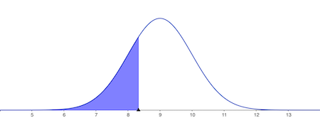
This is an idealized curve. Fred's data roughly resembles this curve. The area under the curve is a probability. Integrating from -∞ to +∞ include all the arrival times, and the probability is 1.
The X on the horizontal axis is the random variable X. We can ask a question like, ''What is the probability the random variable X (i.e., the arrival time) is less than some value?'' In the figure, there is an orange shaded area. This area is the probability the person will arrive less than 5 minutes late. Now, let's ask this type of question in a slightly different way.
Finding the Inverse
Fred would like to know at what time, a, there will be less than 23 members present. This is a probability of 23 / 1,000 = 0.023. Thus, we are asking for the value of X, which will give an area under the curve equal to our given value, or in this case, 0.023. This is the inverse normal probability value. We can write this as P(X < a) = 0.023.
This 0.023 probability is the area under the curve. In principle, we would integrate the normal curve from -∞ to a. The problems are we don't know a, and the integral itself does not have a closed-form solution. We can use numerical methods to approximate the integration very accurately, but we won't have a result as a function of a. If we did, we could set this result equal to 0.023 and use algebra to solve for a.
Also, it would be impossible to tabulate all possible combinations of means and standard deviations. Instead, tables are published for a mean of 0 and a standard deviation of 1. The random variable is called Z. A portion of one of these tables looks like:
 |
Fred looks at the table for the number closest to 0.023. He finds:
- P = 0.0233 for Z = -1.99
- P = 0.0228 for Z = -2.00
- P = 0.0222 for Z = -2.01
Do you see how the numbers in the first column and the numbers in the first row are combined to locate a probability value? We choose the closest: Z = -2.00. Now to relate this value to our bird watchers group.
The relationship between the random variables X and Z:
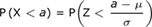 |
In our case, μ = 15 and σ = 5:
 |
Thus, (a - 15) / 5 = -2.00. Solving for a, we get a = 5.
Fred is deliriously happy! He expects to see at least 23 members present after waiting 5 minutes.
The Last Members
Fred wonders at what time everyone will be there except the last 159 members.
 |
This probability is P(X > a). The table, however, describes integration from -∞ to a. We are looking for a. Fred has an idea. Since the total probability is 1, he writes:
 |
And, 1 - P(X > a) = 1 - 0.159 = 0.841.
 |
From the table, 0.841 is closest to 0.8413, which has Z = 1.00. Thus:
(a - 15) / 5 = 1.00 and solving for a we get a = 20.
Thus, at 20 minutes, it is likely all but 159 members will have arrived.
Is There a Quorum?
For this group, a quorum exists when there are 159 members present. Fred wonders if there is an interval of time during which the probability of members present is 0.159. Further, he would like this interval to be centered on the mean.
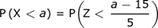
We are looking for P(a < X < b):
 |
In terms of the table, we're looking for:
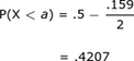 |
and
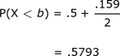 |
This will center the interval about the mean.
From the table:
 |
Thus, (a - 15) / 5 = -0.2, meaning a = 14 and (b - 15) / 5 = 0.2, meaning b = 16.
Fred is happy knowing there will probably be a quorum during the interval 1 minute before and 1 minute after the late arrival time of 15 minutes. Now, if he could only get the birds to be on time!
Lesson Summary
Okay, let's take a brief moment to review the important information that we've learned in this lesson about how to perform an inverse normal probability calculation. We first learned that the bell-shaped curve is the normal probability density function (also known as the Gaussian distribution) and is described by specifying a mean and a standard deviation. The area under the curve of this function, between two points, is the probability a random variable has a value between these two points. When we know the probability and want to find the two points, we're looking for the inverse normal probability. Tables for a mean of 0 and a standard deviation of 1 are numerically computed for the left point being at minus infinity.
Register to view this lesson
Are you a student or a teacher?
Unlock Your Education
See for yourself why 30 million people use Study.com
Become a Study.com member and start learning now.
Become a MemberAlready a member? Log In
BackResources created by teachers for teachers
Over 30,000 video lessons
& teaching resources‐all
in one place.


I would definitely recommend Study.com to my colleagues. It’s like a teacher waved a magic wand and did the work for me. I feel like it’s a lifeline.
Jennifer B.
Teacher

Back

Normal vs. Inverse Normal Distribution | Overview & Formula Related Study Materials
Explore our library of over 88,000 lessons
Browse by subject